Prologue

Transformer Damage Curves (alias: Transformer Capability Curves) are a pretty important thing to have in the reliability industry, since you use them to set your Overcurrent curves. I was recently tasked with generating some of these curves for myself, and found I was disappointed with the current resources on the matter. So, here I am with my own resource to add to the mix.

Note: if you don’t like my coding style or variable naming conventions (Hi, Dr. Dua ;D), you can get over it because I am not a computer programmer.

Resources

If you’ve found this website, it’s probably because you’re researching how to generate these curves on your own. If you’ve been searching for longer than ten seconds, you’ve likely already come across the best resource on the net: https://www.skm.com/applicationguides11.html.

Unfortunately, that website has a bunch of broken formatting, leading me to theorize that the author just copy/pasted from a PDF. Why they didn’t choose to fix it to be actually readable is beyond me, but I’m basically going to regurgitate the information in a way that’s easier to follow.

If you have not, you should reach Chapter 15: Overcurrent Coordination of the IEEE std 242 (IEEE Buff Book), which helps explain why the damage curve for the primary side of the transformer is shifted by 0.58.

Also worth reading is IEEE std C57.109 (IEEE Guide for Liquid-Immersed Transformer Through-Fault-Current Duration) though you will either need to purchase it or have access through your institution. The main thing I got from this standard was that the infrequent damage curves don’t change between transformer categories.

Math

Note: the code I wrote is part of a shared project, so I will not be posting the entirety of the Python since it does not fully belong to me. Between what I post and some quick Chat-GPT, however, you should be able to finish the job.

Open up the SKM resource and follow along. I’m not going to copy and paste their stuff here, just keep their tables in a tab behind the scenes as I will reference them.

For starters, let’s just program the calculations shown in Example 1. (Aside from confusing formatting, I found this example very handy as it was very similar to the transformer that I was actually analyzing in real life).

Declare some variables first. These three variables you will change later, but for now they’re set equal to those found in the example.

1
2
3
4

#Declaration of Variables
XFMR_KVA = 1000 #Needs to be in kVA
XFMR_V_LS = 4.160 #needs to be in kV
XFMR_X = 0.06 #impedance of transformer

Now for some math, following lock-step with the Example:

 1
 2
 3
 4
 5
 6
 7
 8
 9
10
11
12
13
14
15

FLA = (XFMR_KVA)/(1.732*XFMR_V_LS) #Amps at Full Load

I_1800_sec = 2*FLA
I_300_sec  = 3*FLA
I_60_sec   = 4.75*FLA
I_30_sec   = 6.3*FLA
I_10_sec   = 11.3*FLA
I_2_sec    = 25*FLA

I_1800_pri = I_1800_sec*0.58
I_300_pri  = I_300_sec*0.58
I_60_pri   = I_60_sec*0.58
I_30_pri   = I_30_sec*0.58
I_10_pri   = I_10_sec*0.58
I_2_pri    = I_2_sec*0.58

Please note that in the resource, when they say “sec” they mean “seconds” but due to needing different variables for programming, I decided to read “sec” as “secondary” so that I could use “pri” for “primary,” referring, of course, to the secondary and primary side of the transformer.

Note again in the resource how it states that the 0.58 is because it’s a delta-wye transformer. According to example 3, a delta-delta would shift 0.87 instead of 0.58.

1
2
3
4
5
6
7

t = 2551*(XFMR_X*XFMR_X)

I_2_f_sec    = FLA/XFMR_X
I_4_08_f_sec = (0.7*FLA)/XFMR_X

I_2_f_pri    = I_2_f_sec*0.58
I_4_08_f_pri = I_4_08_f_sec*0.58

This above section is where I originally got very confused. For one thing, the resource writes the following:

t 1622 amps = 2551 (0.06)2 = 9.2 seconds

It took me a while to realize it meant this:

t_1622_amps = 2551*(0.06)^2 = 9.2 seconds

where the 2551 is from the table for Class II Transformers. For Class III and IV, replace 2551 with 5000. For Class I, this calculation is not necessary since the frequent fault curve does not shift away from the infrequent fault curve.

The “t” here is important because it determines where on the y-axis (time) your frequent fault curve branches from the infrequent fault curve.

1
2

I_25 = 25*FLA
I_12 = 12*FLA

They also calculate the current inrush though I don’t do much with this personally.

Plotting

So now the fun part, how to plot this? You will need to install matplotlib. This isn’t a python installation tutorial so come back once you’ve got it installed (hint: use pip install).

Slap this at the top of your file:

1

import matplotlib.pyplot as plt

And at the bottom, start with declaring some points for your graph:

1
2
3
4
5
6
7

y_infrequent = [1800,300,60,30,10,2]
y_frequent   = [t, 4.08,2]

x_infrequent_sec = [I_1800_sec,I_300_sec,I_60_sec,I_30_sec,I_10_sec,I_2_sec]
x_infrequent_pri = [I_1800_pri,I_300_pri,I_60_pri,I_30_pri,I_10_pri,I_2_pri]
x_frequent_sec = [I_4_08_f_sec,I_4_08_f_sec,I_2_f_sec]
x_frequent_pri = [I_4_08_f_pri,I_4_08_f_pri,I_2_f_pri]

I’m sure it can be condensed by just multiplying x_infrequent_sec by 0.58 but where’s the fun in that? The more code you write, the better the hacker you are, or something idk.

Please note that the frequent fault x axis arrays are meant to include the current for 4.08 seconds twice as it is the x value for the coordinate pair for t and 4.08.

Now actually plot it:

 1
 2
 3
 4
 5
 6
 7
 8
 9
10
11
12
13
14
15
16
17
18

fig = plt.figure()
ax = fig.add_subplot(1,1,1)
ax.set_title('Equipment Damage Curve')
ax.set_ylabel('Time - sec')
ax.set_xlabel('Current - A')
ax.set_yscale('log')
ax.set_xscale('log')
ax.grid(which = 'both')
ax.set_xlim(left = 10**-1, right = 100000)
ax.set_ylim(bottom = 0.01, top = 10000)
fig.legend(loc = 'upper right')

ax.plot(x_infrequent_sec, y_infrequent, c='b')
ax.plot(x_infrequent_pri, y_infrequent, c='r')
ax.plot(x_frequent_sec, y_frequent, c='b')
ax.plot(x_frequent_pri, y_frequent, c='r')

plt.show()

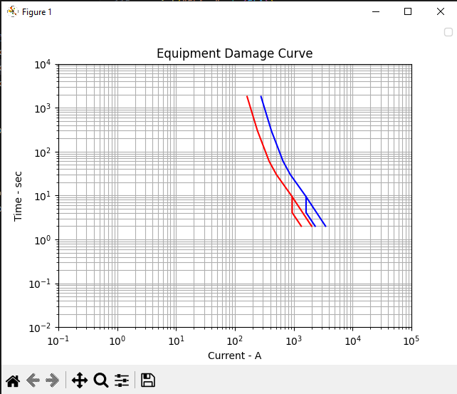
After running your code, you should be presented with this:

Analyzing the graph shows it’s pretty spot-on to the graph shown in the SKM resource.

Note: the graph shown on the SKM resource is scaled at 10^1. This means if you think your generated graph is off by a factor of 10 from the graph in the resource, multiply the x axis in the resource’s graph by 10 and check again (it took me longer than I’d care to admit to catch this, and it caught my coworker as well. Tsk tsk, SKM).

Conclusion

In the end, my coworker and I ended up adding all of the U1-U5 and C1-C5 Overcurrent Protection curves as well. As mentioned earlier, because some of this code belongs to my coworker, I won’t publish it out of respect for his privacy and intellectual property. With that being said, if you want to do the same, you can find the equations for the IEC and U.S. Inverse-Time Overcurrent Curves on page 9 of SEL’s Power System Protection IEC 61131 Library for acSELerator RTAC Projects, among other places, I’m sure. It’s not proprietary or secret knowledge.